Those were the days when an astronomer could still make substantial contributions to mathematics! Bessel functions, first introduced by the German astronomer Friedrich Bessel in the early 19th century, are mathematical functions that arise in various areas of science, engineering, and mathematics. They were and have since become fundamental tools in many fields, including physics, signal processing, and applied mathematics. For Bessel, it was probably mainly the applications in optics, that interested him most: Bessel functions play a crucial role in the study of diffraction, which is the bending or spreading of waves around obstacles or through narrow openings. The diffraction patterns produced by circular apertures or obstacles can be mathematically described using Bessel functions. And to understand diffraction patterns is of course crucial if you want to build better telescopes, as Bessel did.

In this article, we will explore the world of Bessel functions, understand their properties, and learn how to leverage them in Python for practical applications.

$$ x^2 \frac{d^2 y}{d x^2}+x \frac{d y}{d x}+\left(x^2-n^2\right) y=0 $$

x is the independent variable, y is the function we are looking for and n is some real parameter, called the order of the resulting Bessel function. There are many solutions to this equation, but they can be divided into two classes, denoted Jn(x) and Yn(x), called the Bessel functions of the first kind and second kind, respectively.

Before we take a closer look at the useful properties of the Bessel functions, let’s get some intuition how these functions look like. This also gives us a first glimpse into how to use them in Python.

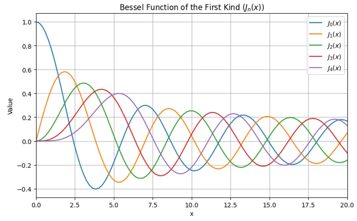
To use Bessel functions in Python, you can leverage the scipy.special module, which provides a wide range of mathematical special functions, including Bessel functions. The relevant functions are aptly called jn and yn. As an example usage, we simplify plot the first few Bessel functions of both kinds:

import numpy as np
import matplotlib.pyplot as plt
from scipy.special import jn, yn

# Define the range of values for the x-axis (argument)
x = np.linspace(0, 20, 100)

# Create subplots
fig, axs = plt.subplots(2, 1, figsize=(8, 10))

for order in range(5):
    
    # Calculate the Bessel functions of the first and second kind
    j_bessel = jn(order, x)
    y_bessel = yn(order, x)

    # Plot Bessel function of the first kind in the first subplot
    axs[0].plot(x, j_bessel, label=f"$J_{order}(x)$")
    
    # Plot Bessel function of the second kind in the second subplot
    axs[1].plot(x, y_bessel, label=f"$Y_{order}(x)$")

# Adjusting design...

axs[0].set_title(f"Bessel Function of the First Kind ($J_n(x)$)")
axs[0].set_xlabel("x")
axs[0].set_ylabel("Value")
axs[0].set_xlim(0, 20)
axs[0].legend()
axs[0].grid(True)

axs[1].set_title(f"Bessel Function of the Second Kind ($Y_n(x)$)")
axs[1].set_xlabel("x")
axs[1].set_ylabel("Value")
axs[1].set_xlim(0, 20)
axs[1].set_ylim(-1, 0.6)
axs[1].legend()
axs[1].grid(True)

plt.tight_layout()

# Show the plot
plt.show()

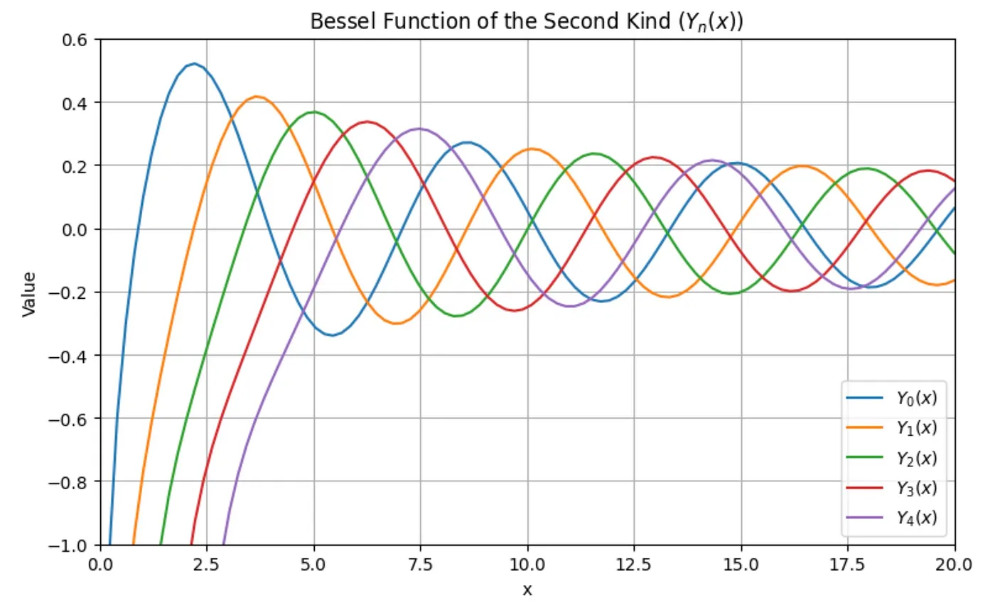
The Bessel functions are usually defined for non-negative values of x. Very roughly speaking, both kinds of Bessel functions look like damped sine or cosine functions. In fact, for large x, they look more and more like these trigonometric functions. But near x=0, the two kinds behave very differently. The first kind is always finite, and in most cases, it starts out from the y=0 at x=0. The only exception is the zero-order (n=0) Bessel function which starts out from 1. The higher the order, the slower the Bessel function starts out from zero. To show this analytically, we can use Python’s sympy package:

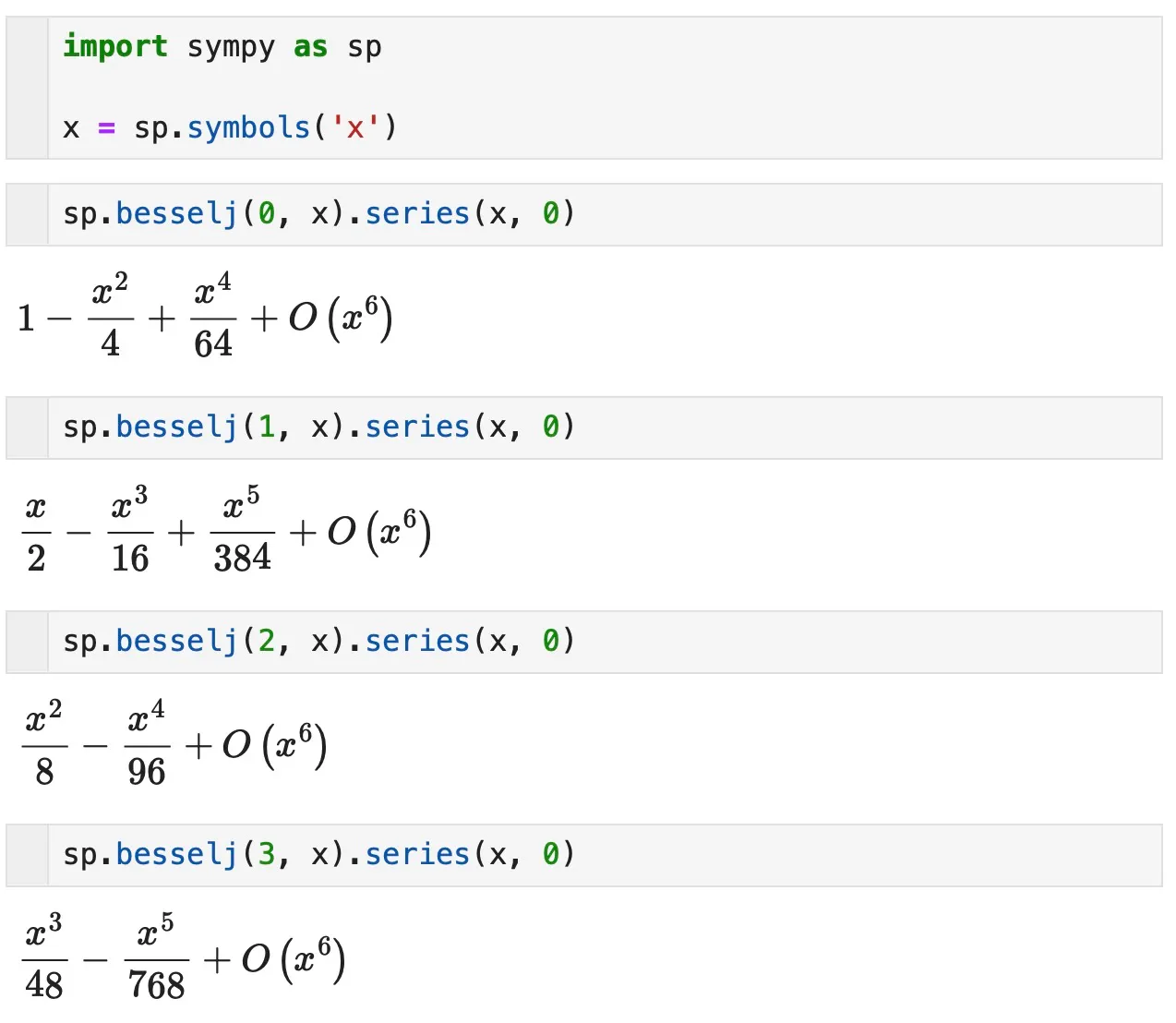
Using sp.besselj() and sp.bessely(), we calculate the Bessel functions of the first and second kind, respectively, and applying the series() method gives us the Taylor expansion at x=0. Obviously, the Bessel function Jn behaves like

$$ J_n(x) \sim x^n $$

as x→0, if n>0.

Not so the Bessel functions of the second kind. The image above shows us that they all go to negative infinity at the origin. Let’s check:

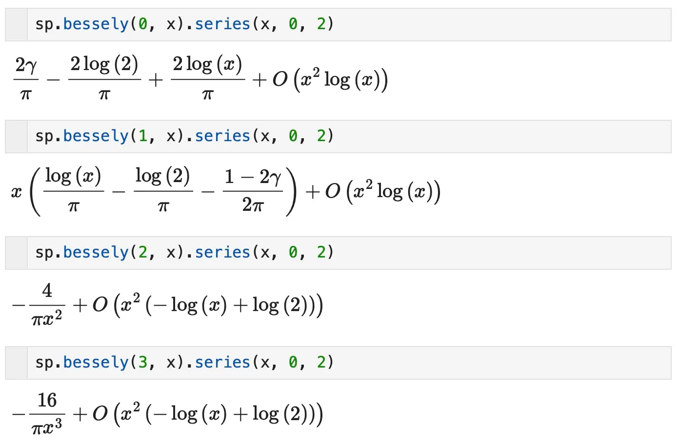
Obviously, the Bessel functions of the second kind are much more unpleasant than those of the first kind. So, when do you need the first and when the second kind? It depends. In general, you need both, because the general solution of the Bessel differential equation is a linear combination of all independent solutions. But in practice, it mostly depends on the use case you have. Often, you can rule out contributions from the Bessel functions of the second kind by applying practical or physical arguments. For instance, solutions with infinite amplitudes are usually not physical so you can simply ignore them (set their coefficient in the linear combination to zero).

Recurrence Relations

Bessel functions satisfy a lot of recurrence relations that facilitate their computation and manipulation. However, one of them has a special status. It is this:

$$ Z_{n-1}(x)+Z_{n+1}(x)=\frac{2 n}{x} Z_n(x) $$

The same recurrence relation holds for J and Y, that’s why I denoted it by the dummy symbol Z, here. Incidentally, this is not the only property of the Bessel functions. In fact, instead of using the Bessel differential equation as a definition, one can instead use this recurrence relation as a definition. I find it quite intriguing that a simple algebraic recurrence relation can have such a rich set of solutions!

Or maybe another simple one, because it relates the Bessel function of positive order to those of negative orders:

$$J_{-n}(x)=(-1)^n J_n(x)$$

But this holds only for integer orders n.

Orthogonality

Orthogonality refers to the property where the inner product (or the integral) of two different functions within a certain interval equals zero, except when the functions are the same. In other words, orthogonal functions are mutually perpendicular in a mathematical sense. This property is similar to the concept of perpendicularity in geometry, where two lines or vectors are at right angles to each other. Examples of orthogonal function sets include the sines and cosines, which have a simple inner product:

$$\int_0^{2 \pi} \sin n x \sin m x= \begin{cases}\pi & \text { if } m=n \\ 0 & \text { otherwise }\end{cases}$$

For Bessel functions, the inner product is a bit more complicated, because it involves a weight. The inner product is

$$\int_0^1 x J_n\left(x x_i\right) J_n\left(x x_j\right) d x= \begin{cases}0 & \text { if } i \neq j \\ \frac{1}{2} J_n^{\prime}\left(x_i\right) & \text { if } i=j\end{cases}$$

where xi and xj are distinct zeros of Jn(x). You see, it’s a lot more complicated than in the case of trigonometric functions. And what are the zeros of the Bessel functions, anyways? They are not equidistant and they can only be computed numerically.

Similarly, Bessel functions of the second kind, Yn(x), exhibit orthogonality with a different weight function, also involving the zeros of Bessel functions.

As these identities are quite complicated, it is not worth memorizing them. But it is important to know that they exist so that you can look them up if you need them.

Other Kinds of Bessel Functions

Bessel functions come in all different sorts and flavors. The first and second kinds are just a start. Depending on your use case, it may be more appropriate to use certain linear combinations of those base kinds to get functions with particularly practical behavior for your use case. For instance, you may often encounter Neumann and Hankel functions. Neumann functions are defined as the combination

$$N_n=\frac{\cos \pi n J_n(x)-J_{-n}(x)}{\sin \pi n}$$

And Hankel functions are linear combinations of first-kind Bessel functions and Neumann functions, e.g.

$$H_n^{ \pm}=J_n(x) \pm i N_n(x)$$

These are also called Bessel functions of the third kind. Note that this is kind of analogous to

$$e^{ \pm i x}=\cos x \pm i \sin x$$

And it doesn’t stop there! There are different sorts of Kelvin functions, and different sorts of Airy functions, all based on the Bessel functions. Again, one doesn’t have to know them by heart, but know that they exist and that they are related to Bessel functions. Then you can always look up the details if the need arises.

Wrapping Up

Bessel functions and their relatives — Neumann, Hankel, Kelvin, and Airy functions — underpin a broad range of scientific and engineering applications. First introduced by Friedrich Bessel, these functions continue to be integral tools in fields as diverse as physics, engineering, and applied mathematics. In this article, we’ve explored the world of Bessel functions, delved into their properties, and learned how to use them in Python.