Recently, I had the problem to find the convex hull of a given set of points. So I to made closer contact with Python's scipy's spatial package. The concept of a convex hull refers to the smallest convex set that contains all the points in a given set. In simpler terms, if you imagine the points as nails in a board, the convex hull would be like a rubber band stretched around the outermost nails, enclosing all the points within. In 2D, you would get a polygon. But the concept not only works in 2D case, but also to higher dimensions. Then you get a body called a simplex.

The 2D Case

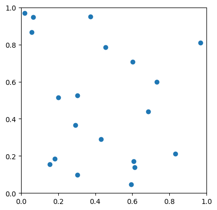
The 2D case represents the scenario where we are dealing with a flat surface and the points lie on a plane. The convex hull in this case is a polygon, and its vertices are connected by straight line segments. Let's start by creating some random points, and visualizing them using a scatter plot.

import matplotlib.pyplot as plt
from scipy.spatial import ConvexHull
import numpy as np

np.random.seed(42)
points = np.random.rand(20, 2)
plt.plot(points[:, 0], points[:, 1], 'o')
plt.xlim(0, 1)
plt.ylim(0,1)
plt.gca().set_aspect("equal")

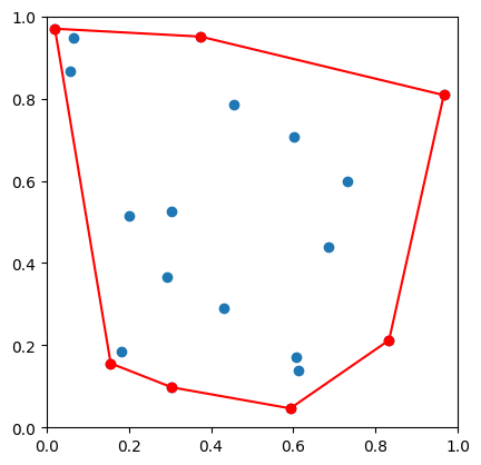
We will now compute the convex hull using scipy's ConvexHull function. This function uses the Quickhull algorithm and provides various attributes to understand and visualize the computed convex hull.

hull = ConvexHull(points)

The vertices property returns the indices of the points that form the vertices of the convex hull. These are the points lying on the outer boundary of the convex hull.

hull.vertices

array([ 5,  2, 18, 14,  6, 17,  0], dtype=int32)

The simplices property provides the indices of the points that make up the simplical facets of the convex hull. In the 2D case, the simplices are just line segments connecting the vertices.

hull.simplices

array([[ 2,  5],
       [ 0,  5],
       [ 0, 17],
       [ 6, 17],
       [ 6, 14],
       [18, 14],
       [18,  2]], dtype=int32)

Next we define a function to plot the hull. The red circles represent the vertices of the convex hull, and the red lines are the line segments forming the boundary.

def plot_hull():
    plt.plot(points[:, 0], points[:, 1], 'o')
    plt.plot(points[hull.vertices][:, 0], points[hull.vertices][:, 1], 'ro')
    for facet in hull.simplices:
        plt.plot(points[facet, 0], points[facet, 1], 'r-')

    plt.xlim(0, 1)
    plt.ylim(0,1)
    plt.gca().set_aspect("equal")
    
plot_hull()

The area attribute refers to the boundary of the hull. So in 2D, the area is actually a length, the perimeter of the hull.

hull.area

3.142052162690126

The volume refers to the interior of the hull. In 2D, the "volume" is actually an area.

hull.volume

0.6449431389347489

For a given facet, we can get the facets that are neighbors of that facet. That's what the neighbors property is for:

hull.neighbors

array([[1, 6],
       [0, 2],
       [3, 1],
       [2, 4],
       [5, 3],
       [4, 6],
       [0, 5]], dtype=int32)

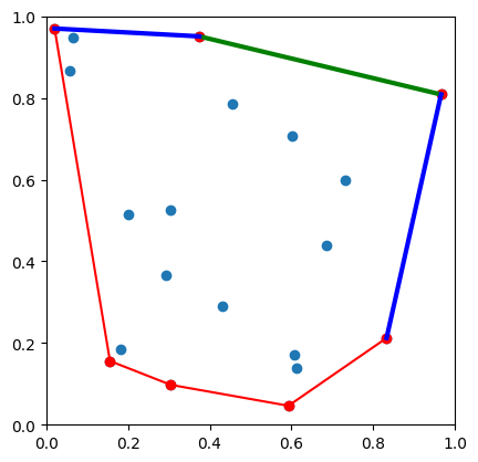
What does that mean? Well, in our example, we have 7 facets with indices from 0 to 6. The output tells us that the neighbor facets of facet 0 are the facets 1 and 6. For facet 1, the neighbor facets are 0 and 2, and so on. In 2D, this is trivial, of course. But not so in higher dimensions any more!

To be clear, let's highlight the facet with index 2 and the neighboring facets.

plot_hull()

# plot the facet with index 2:
facet = hull.simplices[2]
plt.plot(points[facet].T[0], points[facet].T[1], 'g-', lw=3)

# get the indices of the neighboring facets for hull vertex 2: 
neighbor_inds = hull.neighbors[2, :]

# get the point indices for the ends of each neighboring facet:
facets = hull.simplices[neighbor_inds]

for facet in facets:  
    plt.plot(points[facet].T[0], points[facet].T[1], 'b-', lw=3)
    
plt.xlim(0, 1)
plt.ylim(0,1)
plt.gca().set_aspect("equal")

In the plot, we are highlighting the facet with index 2 in green and its neighboring facets in blue.

The 3D Case

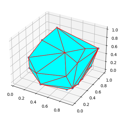
The 3D case represents the scenario where points are in a three-dimensional space. The convex hull in this situation is a polyhedron. The process to compute the convex hull is similar to the 2D case, but now we must deal with three-dimensional facets and vertices.

from mpl_toolkits.mplot3d.art3d import Poly3DCollection

points = np.random.rand(30, 3)

hull = ConvexHull(points)
fig = plt.figure()
ax = fig.add_subplot(111, projection='3d')

# Plot the points
ax.scatter(points[:, 0], points[:, 1], points[:, 2], 'o')

# Plot the convex hull
vertices = [points[face] for face in hull.simplices]
ax.add_collection3d(Poly3DCollection(vertices, facecolors='cyan', linewidths=1, edgecolors='r'))

Here we have generated random 3D points and used scipy's ConvexHull function to calculate the convex hull. We then use matplotlib's 3D plotting functions to visualize the hull as a polyhedron with cyan faces.

The vertices property in 3D gives the indices of the points that form the vertices of the polyhedron, the outer boundary of the convex hull.

hull.vertices

array([ 0,  1,  3,  4,  5,  6,  7,  9, 10, 13, 14, 16, 19, 20, 21, 23, 25,
       26, 27, 28, 29], dtype=int32)

The simplices property provides the indices of the vertices for each triangular facet of the convex hull. In 3D, these facets are triangles forming the faces of the polyhedron.

hull.simplices

array([[ 1,  9, 29],
       [ 0, 25, 10],
       [ 0, 19, 10],
       [ 5, 19, 29],
       [ 5, 19, 10],
       [ 5,  1, 29],
       [ 5,  1,  4],
       [26,  1,  4],
       [26,  1,  9],
       [26,  3,  4],
       [26,  3,  9],
       [21,  0, 25],
       [21, 25,  4],
       [21,  3,  4],
       [27,  5, 10],
       [27,  5,  4],
       [14,  6,  9],
       [14,  9, 29],
       [14, 19, 29],
       [28,  3,  9],
       [28,  6,  9],
       [23,  0, 19],
       [23, 14, 19],
       [23, 14,  6],
       [23,  0, 20],
       [23,  6, 20],
       [ 7, 21,  3],
       [ 7,  0, 20],
       [ 7, 21,  0],
       [16, 25, 10],
       [16, 27, 10],
       [16, 25,  4],
       [16, 27,  4],
       [13,  7, 20],
       [13,  7,  3],
       [13,  6, 20],
       [13, 28,  3],
       [13, 28,  6]], dtype=int32)

Highlight the facet with index 1:

fig = plt.figure()
ax = fig.add_subplot(111, projection='3d')

# Plot the points
ax.scatter(points[:, 0], points[:, 1], points[:, 2], 'o')

# Plot the convex hull
vertices = np.array([points[face] for face in hull.simplices])
ax.add_collection3d(Poly3DCollection(vertices, facecolors='cyan', linewidths=1, edgecolors='r'))
ax.add_collection3d(Poly3DCollection([vertices[1]], facecolors='green', linewidths=1, edgecolors='r'))

In this final plot, we are highlighting a specific facet (with index 1) in green. This type of visualization helps in analyzing specific parts of the hull and can be useful for various geometric and spatial analyses.

Conclusion

The concept of a convex hull is a fundamental notion in computational geometry and has applications across various fields including computer graphics, pattern recognition, image processing, and optimization. This article has illustrated how to compute and visualize convex hulls in both 2D and 3D spaces using Python's scipy.spatial package.