In gravitational physics as well as electrodynamics, there is a problem with arises all too often. This is called Coulomb's problem. In simple words, it is this: suppose you have some distribution of matter in space, like stars in a galaxy or the galaxies in a supercluster, what is corresponding the (Newtonian) gravitational potential? Or stated equivalently: suppose you have some charge distribution in space, what is the corresponding electrostatic potential? In mathematical terms, it reduces to a Poisson equation, but with special boundary conditions:

$$ \nabla^2 \Phi = - 4\pi \rho $$

where \(\Phi\) is the potential and \(\rho\) is the charge or matter distribution. In contrast to normal problem settings with the Poisson equation, the Coulomb problem states the boundary conditions at infinity:

$$ \Phi(|{\bf r}|\rightarrow \infty) = 0 $$

As you can imagine, this is a very common problem, but surprisingly, there are very few ressources in the internet where you can find information how to solve that numerically. In almost all cases, people show how to solve that equation for finite domains, but what about infinite domains like here? That's what we will look at today.

A Pretty Useless Analytic Solution

The Coulomb problem looks innocently simple, but it isn't. It looks so because you can immediately write down the analytic solution, as you can learn in any course on electrodynamics. However, this analytic solution is pretty useless in practice, as we will shortly see.

To see how we can get to this analytic solution, consider the charge in the volume element \(d^3r'\):

$$ Q = \rho({\bf r'})d^3r' $$

This charge in the infinitesimal volume element is like a point charge. So, as we all learned in high school, it generates a Coulomb potential that goes like 1 / distance. So for this volume element we have

$$ d\Phi({\bf r}) = \frac{\rho({\bf r}')d^3r'}{|{\bf r}-{\bf r}'|} $$

To get the total potential, we simply "add up" the contributions from all the other volume elements. We can do that because the Poisson equation is linear:

$$ \Phi({\bf r}) = \int \frac{\rho({\bf r}')d^3r'}{|{\bf r}-{\bf r}'|} $$

This is the analytic solution which automatically satisfies the boundary condition at infinity. But, as I said, it is pretty useless. The reason is that in most interesting cases, the integral cannot be solved analytically. And numerically, it's also problematic, because what we have is actually an integral to solve for each and every point \({\bf r}\) in space! So in practice, we need some other approach.

Numerical Solution

When we solve the normal Poisson equation, we typically have to discretize our finite domain by using some grid. We will do that here, too, even though our boundary conditions seem to require an infinitly large domain. So first of all, we need a method to solve the Poisson equation for some finite domain with some Dirichlet boundary conditions. We will use the Jacobi method here, because it is so simple and stable. It's not a fast method, but one can replace it later by something more fancy like successive over-relaxation or even multigrids.

When we discretize the Laplace operator, we get a the grid point (i, j, k)

$$ \nabla^2 \Phi({\bf r}_{ijk}) \approx \frac{\Phi_{i+1,j,k}+\Phi_{i-1,j,k}+\Phi_{i,j+1,k}+\Phi_{i,j-1,k}+\Phi_{i,j,k+1}+\Phi_{i,j,k-1}-6\Phi_{i,j,k}}{h^2} $$

using 2nd order finite difference. \(h\) is the grid spacing. Note that is again incorporates the idea of the Laplacian being the difference between the local point and the average of the neighborhood.

Inserting this in the Poisson equation and solving for \(\Phi\) at (i, j, k), we get

$$ \Phi_{i,j,k} = \frac{\Phi_{i+1,j,k}+\Phi_{i-1,j,k}+\Phi_{i,j+1,k}+\Phi_{i,j-1,k}+\Phi_{i,j,k+1}+\Phi_{i,j,k-1}- 4 \pi h^2 \rho_{i,j,k}}{6} $$

So this is the recipe, here is the implementation in Python before we look into how to handle the boundary conditions at infinity.

import numpy as np

def jacobi_step(f, rho, h):    
    """Performs a single Jacobi step on the array f and the charge distribution rho."""
    f_new = f.copy()
    f_new[1:-1, 1:-1, 1:-1] = (
          f[2:, 1:-1, 1:-1] + f[:-2, 1:-1, 1:-1] +
          f[1:-1, 2:, 1:-1] + f[1:-1, :-2, 1:-1] +
          f[1:-1, 1:-1, 2:] + f[1:-1, 1:-1, :-2]
          ) + 4*np.pi*rho[1:-1, 1:-1, 1:-1] * h ** 2
    f_new[1:-1, 1:-1, 1:-1] /= 6
    return f_new

Handling the Boundary Conditions

Now, what about the boundary conditions at infinity? Well, we can't have an infinite domain on the computer, so we need a way how to approximate the value of the potential at the boundary. If the grid is reasonably large, we can use the idea presented in my last article: multipoles.

Looking from outside, if you are far enough away from the charge distribution, everything looks like a point charge. If you come closer, you may notice that there is also some dipole present. And as you come closer and closer, you notice more and more contributions from more complex arrangements of virtual point charges. This is the idea of multipoles. So, let's use this multipole approximation to compute the potential at the boundary!

For concreteness, we will use the method of manufactured solutions to get a produce an example which we can easily compare, because by definition we have the exact solution.

This manufactured solution is a smeared out Coulomb potential

$$ \Phi = \frac{{\rm erf}(r/\sigma)}{r} $$

where the smoothing parameter \(\sigma\) cuts off the singularity of the Coulomb potential at \(r=0\). Calculating the Laplacian of that function, we get

$$ \nabla^2 \Phi = -4\pi \frac{e^{-r^2/\sigma^2}}{\pi^{3/2}\sigma^3} $$

As you would expect, our smeared-out Coulomb potential is created by a smeared-out point charge, a Gaussian of width \(\sigma\)!

Now, let's implement that in Python using the multipoles package:

from multipoles import MultipoleExpansion

# Set up the grid
x = y = z = np.linspace(-10, 10, 51)
X, Y, Z = np.meshgrid(x, y, z, indexing="ij")
R = np.sqrt(X ** 2 + Y ** 2 + Z ** 2)

# Set up the charge distribution
rho = np.pi ** -1.5 * np.exp(-R ** 2)

# Calculate the multipole expansion, up to the octopole (l_max=8)
mpe = MultipoleExpansion({'discrete': False, 'rho': rho, 'xyz': (X, Y, Z)}, l_max=8)

# Evaluate the multipole expansion on the boundary of our grid:
boundary = np.ones_like(rho, dtype=bool)
boundary[1:-1, 1:-1, 1:-1] = False

phi = np.zeros_like(rho)
phi[boundary] = mpe[boundary]

Now we have set our boundary and we "just" have to calculate the interior using the Jacobi method. That's what we take care of next.

Putting Things Together

We already have our routine for the Jacobi step and we have also already set the boundary conditions by the multipole expansion. Now we put things together and iterate until convergence:

eps = 1.E-6
max_iter = 10000
h = x[1] - x[0]

for it in range(max_iter):
    phi_new = jacobi_step(phi.copy(), rho, h)
    diff = np.max(np.abs(phi_new - phi))
    if diff < eps:
        break
    phi = phi_new
    it += 1

import matplotlib.pyplot as plt
from scipy.special import erf
R[R==0] = 0.01
phi_ex = erf(R) / R

plt.plot(x, phi_ex[:, 25, 25], label="exact")
plt.plot(x, phi[:, 25, 25], "o", label="numerical")
plt.xlabel("x")
plt.ylabel(r"$\Phi$")
plt.legend();

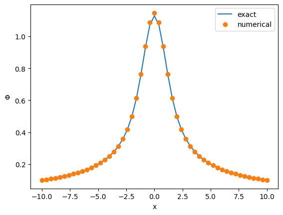
And that's it!