Classical mechanics is the study of the motion of objects under the influence of forces. While it has been around for centuries, classical mechanics is still a fundamental topic in physics and provides a foundation for many other fields of study. One of the most important concepts in classical mechanics is the idea of a system's equations of motion, which can be used to predict the behavior of objects and systems over time.

The double-compound-pendulum is an excellent example of a system with complex motion that can be described using classical mechanics. It consists of two pendulums attached to each other, and the motion of each pendulum affects the other's motion. The double pendulum exhibits chaotic behavior, meaning that small differences in the initial conditions can lead to vastly different trajectories over time.

In this article, we will solve the equations of motion for the double-compound-pendulum in Lagrange mechanics using Python's odeint function. We will then visualize the animated motion of the double pendulum and observe its chaotic behavior.

We can derive the equations of motion using Lagrange mechanics. As described in XXX, all we need is the Lagrangian expressed in our coordinates of choice. The Lagrangian is kinetic energy minus potential energy, which yields

$$ \begin{aligned} & L=\frac{m l^2}{2}\left(\frac{1}{4} \dot{\theta}_1^2+\dot{\theta}_1^2+\frac{1}{4} \dot{\theta}_2^2+\dot{\theta}_1 \dot{\theta}_2 \cos \left(\theta_1-\theta_2\right)\right)+\frac{m l^2}{24}\left(\dot{\theta}_1^2+\dot{\theta}_2^2\right)-m g\left(y_1+y_2\right) \\ & =\frac{1}{6} m l^2\left(\dot{\theta}_2^2+4 \dot{\theta}_1^2+3 \dot{\theta}_1 \dot{\theta}_2 \cos \left(\theta_1-\theta_2\right)\right)+\frac{1}{2} m g l\left(3 \cos \theta_1+\cos \theta_2\right) . \end{aligned} $$

Applying the Euler-Lagrange equations to this Lagrangian gives us the equations of motion:

$$ \begin{aligned} & \dot{\theta}_1=\frac{6}{m \ell^2} \frac{2 p_{\theta_1}-3 \cos \left(\theta_1-\theta_2\right) p_{\theta_2}}{16-9 \cos ^2\left(\theta_1-\theta_2\right)} \\ & \dot{\theta}_2=\frac{6}{m \ell^2} \frac{8 p_{\theta_2}-3 \cos \left(\theta_1-\theta_2\right) p_{\theta_1}}{16-9 \cos ^2\left(\theta_1-\theta_2\right)} . \\ & \dot{p}_{\theta_1}=-\frac{1}{2} m \ell^2\left[\dot{\theta}_1 \dot{\theta}_2 \sin \left(\theta_1-\theta_2\right)+3 \frac{g}{\ell} \sin \theta_1\right] \\ & \dot{p}_{\theta_2}=-\frac{1}{2} m \ell^2\left[-\dot{\theta}_1 \dot{\theta}_2 \sin \left(\theta_1-\theta_2\right)+\frac{g}{\ell} \sin \theta_2\right] \end{aligned} $$

where \(p_{\theta_1}, p_{\theta_2}\) are the conjugated momenta of \(\theta_1\) and \(\theta_2\), respectively.

For convenience, we collect the independent variables in the vector \(\vec y\):

$$ \vec y = (\theta_1, \theta_2, p_{\theta_1}, p_{\theta_2}) $$

so our system of equations obtains the form

$$ \frac{d\vec y}{dt} = f(\vec y) $$

This is the standard form that basically all ordinary differential equation solvers expect. So we write the right hand side of our equation as

g = 9.81
L = 0.5
m = 1

def f(y, t):
    
    dy0_dt = 6.0/(m*L**2) * (2 * y[2] - 3 * np.cos(y[0]-y[1]) * y[3])/(16 - 9 * np.cos(y[0]-y[1])**2)
    dy1_dt = 6.0/(m*L**2) * (8 * y[3] - 3 * np.cos(y[0]-y[1]) * y[2])/(16 - 9 * np.cos(y[0]-y[1])**2)
    dy2_dt = -0.5 * m * L**2 * ( dy0_dt * dy1_dt * np.sin(y[0]-y[1]) + 3 * (g/L) * np.sin(y[0]))
    dy3_dt = -0.5 * m * L**2 * (-dy0_dt * dy1_dt * np.sin(y[0]-y[1]) + (g/L) * np.sin(y[1]))
    
    return [dy0_dt, dy1_dt, dy2_dt, dy3_dt]

We can solve the system of equations using Python's odeint function from the scipy.integrate module. First, we define the function f(y, t) that takes the vector of independent variables y and time t as input and returns the derivative of y with respect to t. We then define the initial conditions y_init, time points t, and call odeint. The output is an array y containing the values of y at each time point. Finally, we can visualize the motion of the double pendulum using matplotlib and observe its chaotic behavior over time:

import numpy as np
from scipy.integrate import odeint

y_init = [np.pi / 2.75, np.pi / 2, 0, 0]

t = np.linspace(0, 50, 2000)
y = odeint(f, y_init, t)

import matplotlib

matplotlib.rcParams["font.size"] = 12
matplotlib.rcParams["lines.linewidth"] = 2

import matplotlib.pyplot as plt

fig, ax = plt.subplots()

ax.plot(t, y[:, 0], label=r"$\theta_1$")
ax.plot(t, y[:, 1], label=r"$\theta_2$")
ax.set_xlabel("time (s)")
ax.set_ylabel("angle (radians)")
ax.legend();

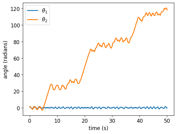
The motion of the double-compound-pendulum can be divided into two regimes. At first, the motion appears oscillation-like, with the pendulums moving back and forth. However, after a short time, the second pendulum flips over, and the motion becomes more unpredictable and non-repeating. The double pendulum exhibits chaotic behavior, which means that small differences in the initial conditions can lead to vastly different trajectories over time. In the case of the double pendulum, the chaotic behavior arises due to the nonlinear coupling between the two pendulums. This type of behavior is common in many physical systems and has important applications in fields such as weather prediction and stock market analysis.

We can animate the motion of the double pendulum using matplotlib's animation function:

from matplotlib import animation

%matplotlib notebook

fig, ax = plt.subplots(figsize=(5,5))

ax.set_xlim([1, -1])
ax.set_ylim([-1.5, 0.5])

plt.axis("off")

dt = t[1] - t[0]

pendulum_1, = ax.plot([], [], "r")
pendulum_2, = ax.plot([], [], "b")

def init():
    pendulum_1.set_data([], [])
    pendulum_2.set_data([], [])

def animate(frame): 
    ax.set_title("Time: %10.2f s" % (frame * dt))
    x_1 = L * np.sin(y[frame, 0])
    y_1 = - L * np.cos(y[frame, 0])
    x_2 = x_1 + L * np.sin(y[frame, 1])
    y_2 = y_1 - L * np.cos(y[frame, 1])
    
    pendulum_1.set_data([0, x_1], [0, y_1])
    pendulum_2.set_data([x_1, x_2], [y_1, y_2])
    return [pendulum_1, pendulum_2]

    
anim = animation.FuncAnimation(fig, animate, frames=len(t), interval=20)

After about 5 seconds, the second pendulum flips over several times.

The function animate updates the position of the pendulums at each time step, and the FuncAnimation class creates an animation from these updates. We can observe the chaotic behavior of the double pendulum as the second pendulum flips over several times, making it challenging to predict the motion accurately. This behavior is due to the system's nonlinear dynamics, where small changes in the initial conditions can lead to significant differences in the pendulums' trajectories. The double-compound-pendulum is one of the simplest examples of a chaotic system in classical mechanics and demonstrates the importance of understanding the behavior of nonlinear systems.

Conclusion

In conclusion, the double-compound-pendulum is a fascinating system that exhibits chaotic behavior in classical mechanics. We derived the equations of motion using Lagrange mechanics and solved them using Python's odeint function. We visualized the motion of the double pendulum using matplotlib and observed the complex and unpredictable behavior that arises due to the system's nonlinear dynamics.