Today, we will be discussing a crucial aspect of numerical computing — efficient matrix construction in numpy . Matrix operations are the backbone of many scientific and engineering applications and play a crucial role in machine learning algorithms. Numpy provides a convenient and efficient platform to perform matrix operations, but building matrices can still be a challenge. In this blog post, we will explore how to create complicated matrices with the help of numpy’s vectorization features, avoiding the slow process of looping over rows and columns. By the end of this post, you will have a good understanding of how to create matrices efficiently in numpy and apply this knowledge to various applications. So, let’s dive in!

Our sample matrix

Suppose we want to create a complicated (N+1)×(N+1) matrix D in Python with the following entries:

$$ \begin{aligned} &D_{00}=\frac{2 N^2+1}{6} \quad D_{N N}=-\frac{2 N^2+1}{6}\\ &\begin{gathered} D_{j j}=-\frac{x_j}{2\left(1-x_j^2\right)} \quad j=1, \ldots, N-1 \\ D_{i j}=\frac{c_i}{c_j} \frac{(-1)^{i+j}}{x_i-x_j} \quad i \neq j, \quad i, j=0, \ldots N \end{gathered} \end{aligned} $$

where

and

If you are wondering what this matrix describes, here it is: it's the Chebyshev differentiation matrix, a spectral representation of the derivative operator on a Chebyshev grid. We will see an example of its application at the end of this article.

The naive approach to build the matrix would be to create an empty 2D array and loop over rows and columns:

# The naive way. Don't do this!

import numpy as np

N = 30
D = np.zeros((N+1, N+1))

for i in range(N+1):
    for j in range(N+1):
        ...

However, as you may know, this is a very bad idea because for loops are notoriously slow in Python. That's why you should use the vectorization features of numpy instead. For a complicated matrix like this where you have a recipe in terms of row and column indices, you have to pull some numpy tricks, though. That's what we are going to do now.

Efficient matrix construction

Let's start with the vector xⱼ . For concreteness and to keep output short, we will choose N=3.

import numpy as np

N = 3

x = np.cos(np.pi * np.arange(N+1) / N)

array([ 1. ,  0.5, -0.5, -1. ])

Ok, so it looks like numpy treats x as a row vector. We will see in a minute that this is NOT the case. But for now, let's turn to the next step. I would like to define a matrix X with indices

$$ X_{i j}=x_i-x_j \quad i, j=0, \ldots, N $$

How can we do this in numpy ? Well, we can hope that numpy behaves intuitively. If so, I would expect that I could take the difference between x and its transpose and hope that it automatically inflates the vectors to a matrix. Let's try:

x - x.T

array([0., 0., 0., 0.])

Nope, it's still a vector, but why? Let's inspect the shape of x :

x.shape

(4,)

This means that it is not a row vector at all. If that was the case, the shape would have to be (1, 4) . It's not a column vector either, because then the shape would be (4, 1) instead of (4,) . So, we should memorize that constructing a "vector" in numpy creates neither a row nor a column vector. If we want such vectors, we need to explicitly say so, by using reshape , for example:

x = x.reshape(1, N+1)  # turn x into a row vector

x.shape

(1, 4)

x = x.reshape(N+1, 1) # turn x into a column vector
x

array([[ 1. ],
       [ 0.5],
       [-0.5],
       [-1. ]])

Then the inflation works as expected:

X = x - x.T

array([[ 0. ,  0.5,  1.5,  2. ],
       [-0.5,  0. ,  1. ,  1.5],
       [-1.5, -1. ,  0. ,  0.5],
       [-2. , -1.5, -0.5,  0. ]])

Now we can try to create the off-diagonal entries of our matrix D:

$$ D_{i j}=\frac{c_i}{c_j} \frac{(-1)^{i+j}}{x_i-x_j} \quad i \neq j, \quad i, j=0, \ldots N $$

The idea is to create two more matrices C and S with entries

and

so that we can write

We define

c = np.ones_like(x)
c[0, 0] = c[0, -1] = 2

array([[2.],
       [1.],
       [1.],
       [1.]])

By using ones_like we don't have to explicitly reshape to get a row vector, because the _like inherits the shape from x which we have already defined to be a column vector.

c.shape

(4, 1)

C = c / c.T

array([[1. , 2. , 2. , 2. ],
       [0.5, 1. , 1. , 1. ],
       [0.5, 1. , 1. , 1. ],
       [0.5, 1. , 1. , 1. ]])

Now for the sign matrix:

j = np.arange(N+1).reshape(N+1, 1)

S = (-1)**j * (-1)**j.T
S

array([[ 1, -1,  1, -1],
       [-1,  1, -1,  1],
       [ 1, -1,  1, -1],
       [-1,  1, -1,  1]])

Now we are ready to define the off-diagonal entries of D. Almost. We still need to pick out the off-diagonal entries of the matrix. If we just write

D = C * S / X

we get an error because we also selected the diagonal entries and the xᵢ − xⱼ in the denominator for i=j is zero. So we must use a mask to pick the off-diagonal entries. It's easier to define a mask for the diagonal entries first, and then invert it by negation.

mask_diag = np.eye(N+1, dtype=bool)

array([[ True, False, False, False],
       [False,  True, False, False],
       [False, False,  True, False],
       [False, False, False,  True]])

Now simply invert:

mask_off = ~mask_diag

array([[False,  True,  True,  True],
       [ True, False,  True,  True],
       [ True,  True, False,  True],
       [ True,  True,  True, False]])

D = np.zeros((N+1, N+1))

D[mask_off] = C[mask_off] * S[mask_off] / X[mask_off]

array([[ 0.        , -4.        ,  1.33333333, -1.        ],
       [ 1.        ,  0.        , -1.        ,  0.66666667],
       [-0.33333333,  1.        ,  0.        , -2.        ],
       [ 0.25      , -0.66666667,  2.        ,  0.        ]])

Now for the diagonal entries

$$ D_{j j}=-\frac{x_j}{2\left(1-x_j^2\right)} \quad j=1, \ldots, N-1 $$

When applying the diagonal mask to D , we get a 1D array with a reference to all the diagonal entries (which are all 0 right now). So for the right-hand side we also need a 1D array. But x is 2D right now because we had turned it into a column vector of shape (4, 1) . So we have to undo this at this point, using reshape(-1) . And of course, we must not use all values but just the ones with indices 1…,N−1:

x = x.reshape(-1)     # turns x back into shape (N,)

diag = np.zeros(N+1)
diag[1:-1] = - x[1:-1] / (2*(1-x[1:-1]**2))

D[mask_diag] = diag

array([[ 0.        , -4.        ,  1.33333333, -1.        ],
       [ 1.        , -0.33333333, -1.        ,  0.66666667],
       [-0.33333333,  1.        ,  0.33333333, -2.        ],
       [ 0.25      , -0.66666667,  2.        ,  0.        ]])

All that remains is the 2 entries on the upper left and lower right corner:

D[0, 0] = 2*(N**2 + 1) / 6
D[N, N] = - D[0, 0]

And we are done:

array([[ 3.33333333, -4.        ,  1.33333333, -1.        ],
       [ 1.        , -0.33333333, -1.        ,  0.66666667],
       [-0.33333333,  1.        ,  0.33333333, -2.        ],
       [ 0.25      , -0.66666667,  2.        , -3.33333333]])

Let's put that all in a function:

def cheb(N):
    
    x = np.cos(np.pi * np.arange(N+1) / N)
    x = x.reshape(1, N+1) 
    X = x - x.T
    
    c = np.ones_like(x)
    c[0, 0] = c[0, -1] = 2
    C = c / c.T
    
    j = np.arange(N+1).reshape(1, N+1)
    S = (-1)**j * (-1)**j.T
    
    mask_diag = np.eye(N+1, dtype=bool)
    mask_off = ~mask_diag

    D = np.zeros((N+1, N+1))
    D[mask_off] = C[mask_off] * S[mask_off] / X[mask_off]

    x = x.reshape(-1)     # turns x back into shape (N,)

    diag = np.zeros(N+1)
    diag[1:-1] = - x[1:-1] / (2*(1-x[1:-1]**2))

    D[mask_diag] = diag
    D[0, 0] = (2*N**2 + 1) / 6
    D[N, N] = - D[0, 0]
    return D.T

Example Application

Now let's apply the matrix function we have just created. As promised in the beginning, the matrix is a representation of a derivative operation on a Chebyshev grid. So let's put a function on such a grid and compare its exact derivative with that computed with the Chebyshev matrix. We will do that for different numbers of grid points so that we can see the scaling behavior:

import matplotlib.pyplot as plt


Ns = np.logspace(1, 2, 30, dtype=int)
errs = []

for N in Ns:    
    x = np.cos(np.arange(N+1)*np.pi/N)
    f = np.exp(-x**2) + x
    df_dx_exact = -2*x*np.exp(-x**2) + 1
    
    D = cheb(N)
    df_dx = np.dot(D, f)
    err = np.max(np.abs(df_dx - df_dx_exact))
    errs.append(err)
    
plt.loglog(Ns, errs, '-o')
plt.grid()
plt.xlabel('N')
plt.ylabel('max. error in derivative');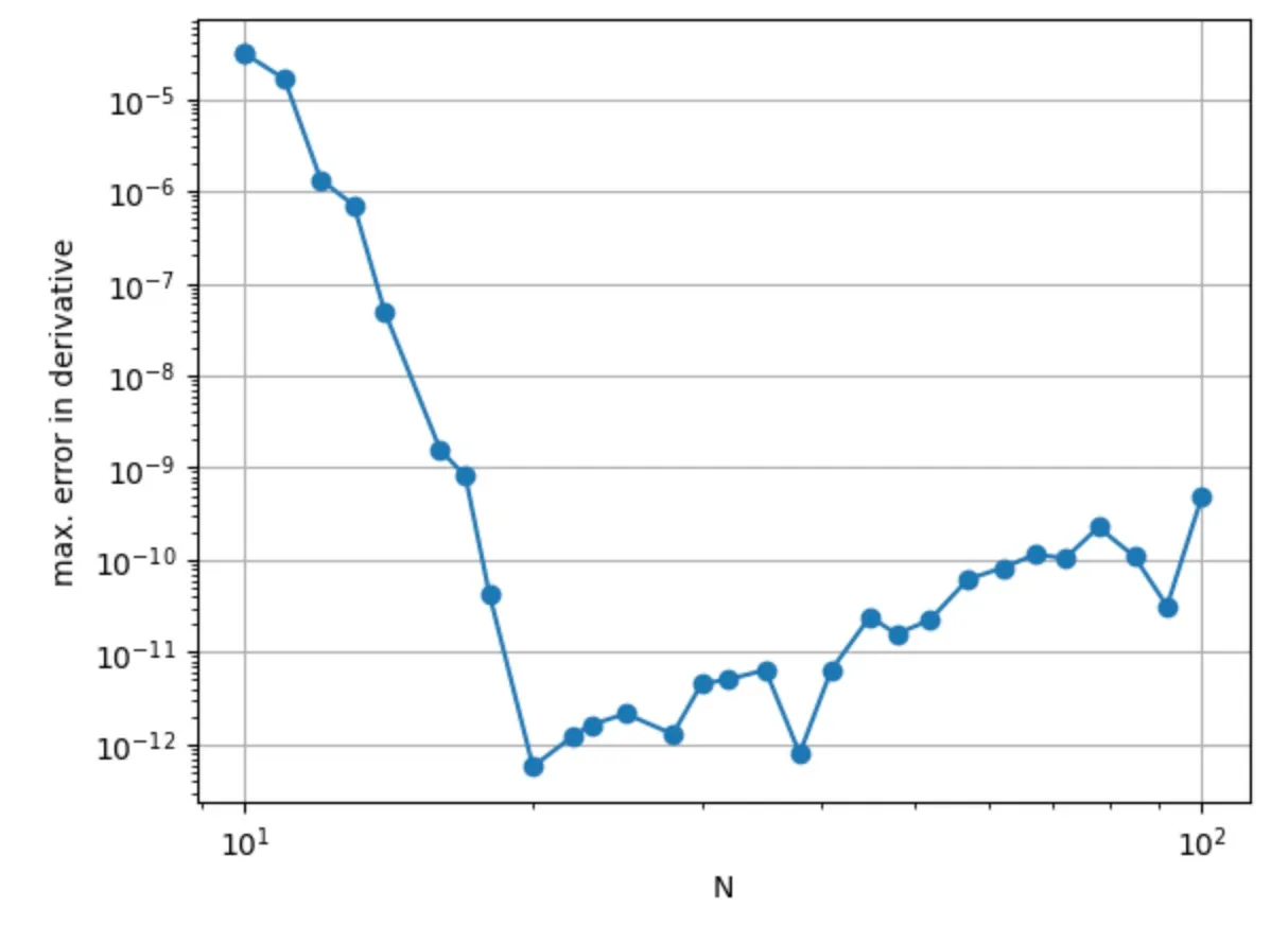

With only 20 grid points, we have already reached a precision of 10⁻¹²! That's the famous spectral accuracy!

Conclusion

In conclusion, we have seen how to efficiently construct a complicated matrix in numpy , taking advantage of its vectorization features to speed up the process. By using numpy tricks and understanding the behavior of numpy arrays, we were able to build the Chebyshev differentiation matrix, a useful tool in various applications such as numerical differentiation and solving differential equations. We hope that this blog post has provided valuable insights for those who seek to optimize their code and improve their matrix construction skills. Until next time, happy coding!