In today's article, we'll cover a counterintuitive, seemingly paraxodical physical effect, how to use event-triggered termination of ordinary differential equation solving on Python, and all along some practice in Lagrangian mechanics.

The effect is this: Consider an object falling freely from height \(L\). When it hits the ground, it has some velocity. So far, nothing special. Now consider a tower of height \(L\), falling freely to the side. Does the tower have the same velocity when it hits the ground? Spontaneously, out of reflex (thinking of Galileo), I would have said: yes. But closer examination shows that this is not at all the case. And what's even more intruiguing: The tower is faster! Let's see why.

Free Fall

First of all, let's treat the object falling freely from height \(y = L\). To calculate its velocity when it hits the ground, we simply invoke energy conservation. Initially, when at height \(L\), the object has zero velocity, so its kinetic energy is zero and the potential energy is simply \(m g L\). So we have

$$ E = m g L $$

When it hits the ground, it has zero potential energy (because the height \(y\) is now 0) and the total energy is just from kinetic energy. So we have

$$ E = \frac{m}{2}v^2. $$

Solving for \(v\), we get

$$ v = \sqrt{2 g L} $$

That was all too easy. So now let's consider this other, curious example.

Falling Tower

Consider a "tower", and suppose it is falling to the side. What we want to calculate is this: When the tower hits the ground, what is the speed of the top of the tower?

The problem can be easily solved using Lagrangian mechanics. If you want to brush up on this topic, have a look at this article .

In Lagrangian mechanics, we basically just have to choose the most convenient coordinates and then formulate the Lagrangian, which is simply the difference of kinetic and potential energy, expressed in our coordinates of choice. Then we solve the corresponding socalled Euler-Lagrange equations. So, here it goes.

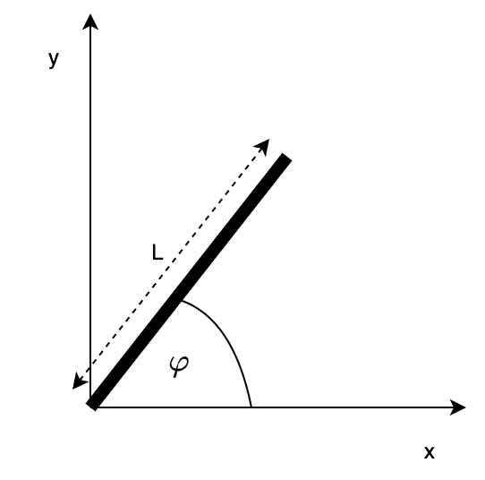
The most convenient coordinate is the angle between the ground and the tip of the tower. When it is \(\varphi=\pi/2\), the tower is still standing, when it is \(\varphi = 0\), the tower is on the ground.

We will consider the tower as one-dimensional with constant linear mass density \(\mu\). So, a line element \(dl\) along the tower has the mass \(dm=\mu dl\). The line element is at height \(y = l \).

Line element \(dl\) at length \(l\) away from origin is at height \(l \sin \varphi\), so it has potential energy

$$ dV = \mu l \sin \varphi dl $$

The total potential energy of the tower is then just then integral

$$ V = \mu g \sin\varphi \int_0^L l dl = \frac{1}{2} g \mu L^2\sin\varphi $$

The velocity of each line element can only have a component perpendicular to the tower. So the kinetic energy is

$$ T = \frac{\mu}{2} \int_0^L l^2 \dot \varphi^2 dl = \frac{\mu}{6}\dot\varphi^2 L^3 $$

So, we get our Lagrangian as

$$ L = T - V = \frac{1}{2}\mu L^2 \sin\varphi - \frac{1}{6}\mu g \dot \varphi^2 L^3 $$

From this we can evaluate the equation of motion, the Euler-Lagrange equation:

$$ \frac{d}{dt}\frac{\partial L}{\partial \dot \varphi} = \frac{\partial L}{\partial \varphi} $$ $$ \frac{1}{3}\mu \ddot \varphi L^3 = -\frac{1}{2}\mu g L^2 \cos\varphi $$

Solving for the angular acceleration, we get

$$ \ddot \varphi = -\frac{3g}{2L} \cos\varphi $$

This is what we need to solve. It can't be done analytically, so we solve it numerically using Python. To do this, we have to bring our equation into standard form

$$ \frac{dY}{dt} = f(Y, t) $$

Simply define

$$ Y = \left(\varphi, \dot \varphi \right) $$

and our equation can be written as

$$ \frac{dY}{dt} = \left(Y_1, -\frac{3g}{2L}\cos Y_0\right) $$

We want to solve that with scipy's ODE solver. But there's a catch. Normally, when we are solving an initial value problem like this, we ask the solver to give us the solution from time t=0 to some fixed time t_end. But what is t_end? Well, it's the time when the tower hits the ground, but we don't know what its numeric value is, yet! How can we tell the solver what we want it to do? Look at the signature of the solve_ivp function from scipy:

scipy.integrate.solve_ivp(fun, t_span, y0, method='RK45', t_eval=None, dense_output=False, events=None, vectorized=False, args=None, **options)

What we need is the events keyword. We can tell the solver that it look for certain events while solving the problem. And if we do so, we solver will remember when and under what conditions these events occur. In our case, the event we are interested in is when the tower hits the ground, so when \(\varphi = 0\). The events keyword wants a callable (or a list of callables, if we want to watch more than just one event). Each callable must be of the form event(t, y) and must return a float value. The solver will insert the current time and current value at each step and evaluate that function. If it returns 0, the event triggers, if it is not equal to zero, it does not trigger. In our case, we want it to trigger, when \(\varphi=0\), and \(\varphi\) corresponds to y[0]. So we write

def termination_event(t, y):
    return y[0]

We could pass that to the solver, but then it would just record when this event fires. It would not terminate integration. However, we can tell it to do so. We just have to attach a property called terminal to the callable:

def termination_event(t, y):
    return y[0]

termination_event.terminal = True

With this in place, we can now use the solver:

from scipy.integrate import solve_ivp

L = 30 # meters
g = 9.81 # Earth gravitational constant in m / s**2

def f(t, y):
    phi = y[0]
    return [y[1], -1.5 * g/ L * np.cos(y[0])]
            
# we have to give it a little "push", otherwise it will stand still
eps = 1.E-3
y_init = [np.pi / 2-eps, 0]

sol = solve_ivp(f, (0, 100), y_init, events=termination_event)

sol

  message: 'A termination event occurred.'
     nfev: 56
     njev: 0
      nlu: 0
      sol: None
   status: 1
  success: True
        t: array([ 0.        ,  0.12358769,  1.35946458,  3.08561937,  5.09644608,
        7.26957071,  9.50476927, 11.36693393, 11.57346943])
 t_events: [array([11.57346943])]
        y: array([[ 1.56979633e+00,  1.56979258e+00,  1.56930767e+00,
         1.56639830e+00,  1.55303743e+00,  1.48953264e+00,
         1.18323312e+00,  1.94766909e-01, -1.66533454e-16],
       [ 0.00000000e+00, -6.06954721e-05, -7.72185329e-04,
        -2.99905727e-03, -1.24172381e-02, -5.68932738e-02,
        -2.69723190e-01, -8.90414682e-01, -9.92405607e-01]])
 y_events: [array([[-1.66533454e-16, -9.92405607e-01]])]

Let's have a look at what this output means. The message indicates that the solver has found our termination condition. That's good. This termination condition occurred at time \(t=11.5737s\) (t_events). At this time, the solution was

 y_events: [array([[-1.66533454e-16, -9.92405607e-01]])]

The first argument is \(\varphi\), the second is the angular velocity at that time. Our terminal speed is then

$$ v = L \dot \varphi $$

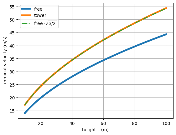
Let's compare this with the terminal velocity for free fall, and let's look at the dependency on \(L\).

import numpy as np
import matplotlib.pyplot as plt

Ls = np.linspace(10, 100, 100)
vs = []

for L in Ls:
    
    def f(t, y):
        phi = y[0]
        return [y[1], -1.5 * g / L * np.cos(y[0])]
    
    sol = solve_ivp(f, (0, 100), y_init, events=termination_event)
    if sol.y_events:
        v = abs(L * sol.y_events[0][0, 1])
        vs.append(v)
    else:
        print(L, "did not succeed")

vs = np.array(vs)  
vs_free = np.sqrt(2*g*Ls)

plt.plot(Ls, vs_free, lw=4, label="free")
plt.plot(Ls, vs, lw=4, label="tower")
plt.plot(Ls, vs_free * np.sqrt(3/2), "-.", lw=2, label=r"free $\cdot \sqrt{3/2}$")
plt.xlabel("height L (m)")
plt.ylabel("terminal velocity (m/s)")
plt.legend()
plt.grid()

As you can see, the tip of the tower always has a higher speed than an object falling freely from the same height. By how much? That's why I also plotted the curve for free fall, scaled by a factor of \(\sqrt{3/2}\), and it's right on top of the curve for the tower. So, as a result, we now know the analytic expression for the terminal speed of the tip of the tower. It's

$$ v = \sqrt{3 gL} $$