In the world of mathematics, every so often, we stumble upon ingenious theorems that leave us marveling at the elegance and simplicity with which they solve problems. One such gem is Pick's theorem—a remarkably simple method for calculating the area of any polygon with vertices lying on lattice points of a grid. In this blog post, we will see how this works. Pick's theorem is named after Austrian mathematician Georg Alexander Pick, who first published the theorem in 1899. It has since found applications in various areas of mathematics, such as combinatorial geometry and number theory.

Pick's Theorem Formula

Given a simple polygon P with vertices on the lattice points of a grid, the area A of the polygon can be calculated using the formula:

$$ A = I + \frac{B}{2} - 1 $$

where \(A\) is the area of the polygon, \(I\) is the number of lattice points located inside the polygon, \(B\) is the number of lattice points located on the boundary (edges and vertices) of the polygon. Note that Pick's theorem only works for simple polygons, meaning those that do not have self-intersections.

import numpy as np
import matplotlib.pyplot as plt

def plot_polygon_on_grid(ax, vertices, boundary, interior):
    
    for i in range(-1, 10):
        ax.axhline(i, color='gray', linewidth=0.5)
        ax.axvline(i, color='gray', linewidth=0.5)
        
    polygon = plt.Polygon(vertices, fill=None, edgecolor='black', linewidth=2)
    ax.add_patch(polygon)
    if boundary:
        ax.scatter(*zip(*boundary), marker='o', color='red', zorder=10)
    if interior:
        ax.scatter(*zip(*interior), marker='o', color='blue', zorder=10)
    
    ax.set_aspect('equal')
    plt.xticks(np.arange(-1, 10, 1))
    plt.yticks(np.arange(-1, 10, 1))
    plt.xlim(-1, 6)
    plt.ylim(-1, 6)
    plt.grid(True)
    plt.show()
    return ax

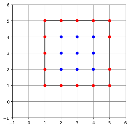
Let's first consider a very simple case, for which we actually don't have to invoke a theorem: a square. Take the vertices (1,1), (1,5), (5,5), and (5,1):

fig, ax = plt.subplots()
vertices = [(1, 1), (1, 5), (5, 5), (5, 1)]
boundary = [
    (1, 1), (1, 2), (1, 3), (1, 4), (1, 5),
    (2, 5), (3, 5), (4, 5), (5, 5), (5, 4),
    (5, 4), (5, 2), (5, 1), (4, 1), (3, 1), (2, 1)
]
interior = [
    (2, 2), (2, 3), (2, 4), (3, 4), (4, 4),
    (4, 3), (4, 2), (3, 2), (3, 3)
]
plot_polygon_on_grid(ax, vertices, boundary, interior)

Obviously, it's a square of side length 4, so the area is simply 16.

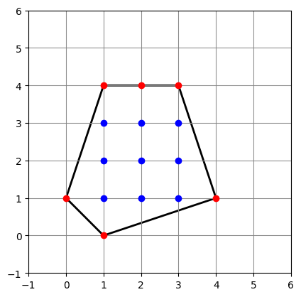
Now let's use Pick's theorem. The polygon has 9 interior lattice points (\(I = 9\)). There are 16 lattice points on the boundary, including the vertices (\(B = 12\)). So we have \(A = 9 + 8 - 1 = 16\). Ok, that was easy and we didn't actually require Pick's theorem to calculate the area of a square. But what about this one:

fig, ax = plt.subplots()

vertices = [(0, 1), (1, 0), (4, 1), (3, 4), (1, 4)]
boundary = [
    (1, 4), (2, 4), (3, 4),
    (4, 1), (1, 0), (0, 1)
]
interior = [
    (1, 1), (1, 2), (1, 3), (2, 3), (3, 3),
    (3, 2), (3, 1), (2, 1), (2, 2)
]

plot_polygon_on_grid(ax, vertices, boundary, interior)

According to Pick's theorem, we have

$$ A = 9 + 6 / 2 - 1 = 11 $$

But is that correct?

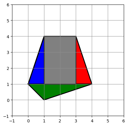
Let's double check and calculate it by hand. The idea is that every polygon on the grid can be split into rectangles and triangles. In our case, it looks like this:

fig, ax = plt.subplots()

for i in range(-1, 10):
    ax.axhline(i, color='gray', linewidth=0.5)
    ax.axvline(i, color='gray', linewidth=0.5)

polygon = plt.Polygon(vertices, fill=None, edgecolor='black', linewidth=2)
ax.add_patch(polygon)



triangle = np.array([(1, 4), (1, 1), (0, 1)])
ax.fill(*triangle.T, facecolor="blue", edgecolor='black', linewidth=2)

triangle = np.array([(3, 1), (3, 4), (4, 1)])
ax.fill(*triangle.T, facecolor="red", edgecolor='black', linewidth=2)

triangle = np.array([(4, 1), (1, 0), (0, 1)])
ax.fill(*triangle.T, facecolor="green", edgecolor='black', linewidth=2)

rect = np.array([(1, 1), (1, 4), (3, 4), (3, 1)])
ax.fill(*rect.T, facecolor="gray", edgecolor='black', linewidth=2)

ax.set_aspect('equal')
plt.xticks(np.arange(-1, 10, 1))
plt.yticks(np.arange(-1, 10, 1))
plt.xlim(-1, 6)
plt.ylim(-1, 6)
plt.grid(True)
plt.show()

The area of the gray rectangle is \(2 x 3 = 6\). The area of the blue triangle is

$$ \frac{1}{2} \cdot 1 \cdot 3 = \frac{3}{2} $$

For the green triangle we have

$$ \frac{1}{2} \cdot 1 \cdot 4 = 2 $$

and the red triangle has the same are as the blue one. So in total, we have

$$ A = 6 + 2 + 2 \frac{3}{2} = 11 $$

in agreement with Pick's theorem. But Pick's theorem applies for the most general case. For all polygons with all orientations, and such a simple formula. Amazing, isn't it?