Stars are colossal spheres of hot gas that undergo nuclear fusion in their cores. To understand the properties and behaviors of stars, astronomers and astrophysicists often apply various models to study their structure. Among the most useful models is the polytropic model, which simplifies the complicated physics inside a star into a more manageable form.

The concept of polytropic stars dates back to the early 20th century, and the model has become a fundamental tool in stellar astrophysics. Using a polytropic equation of state, this model incorporates critical variables such as pressure, density, mass, and radius. By understanding how these variables interact, we can derive essential insights into the star's life cycle, stability, and physical characteristics. At that time, solving these models meant a tremendous amount of work. But today with computing power at our finger tips, everyone can do it.

This tutorial provides an explanation how to calculate the structure of polytropic stars using the Python programming language. We will derive and solve the key equations describing the star's structure, namely the mass continuity equation and the hydrostatic equilibrium equation, and use numerical methods to find solutions that represent different types of stars. The polytropic model, while an approximation, can capture the behavior of various stellar objects, from main sequence stars to white dwarfs.

Mass Continuity Equation

The first equation we'll derive is the mass continuity equation, which describes how mass is distributed within a spherically symmetric star or planet. This equation arises from considering the fundamental relationship between density, volume, and mass.

Consider a thin spherical shell at a radius \(r\) within the object, having a thickness \(dr\). The volume of this shell is given by the surface area of the sphere, \(4\pi r^2\), multiplied by the thickness, \(dr\). If we multiply this volume by the density, \(\rho(r)\), we get the mass of the shell, \(dM(r)\):

$$ dM(r) = 4\pi r^2 \rho(r) dr $$

Dividing both sides of this equation by \(dr\), we arrive at the mass continuity equation:

$$ \frac{dM(r)}{dr} = 4 \pi \rho(r) r^2 $$

This equation tells us how the enclosed mass changes as we move outward from the center of the object.

Hydrostatic Equilibrium Equation

The second equation, known as the hydrostatic equilibrium equation, describes the balance of forces within the object. Specifically, it tells us how the gravitational force is balanced by the pressure gradient force, ensuring that the object maintains its shape and does not collapse under its own gravity.

To derive this equation, we start by considering the gravitational force on the same mass element we considered earlier. Using Newton's law of gravitation, the gravitational force on this element due to the enclosed mass, \(M(r)\), is:

$$ dF_{\text{gravity}} = \frac{G \, dm \, M(r)}{r^2} $$

Substituting our expression for \(dm\) from the mass continuity equation, we find:

$$ dF_{\text{gravity}} = \frac{G \, M(r) \, 4\pi r^2 \rho(r) dr}{r^2} $$

Next, we consider the pressure gradient force. This force arises from the pressure differential across the mass element, and it acts outward, opposing the gravitational force. It's given by:

$$ dF_{\text{pressure}} = - dP \, 4\pi r^2 $$

In hydrostatic equilibrium, these forces must be balanced:

$$ dF_{\text{gravity}} = dF_{\text{pressure}} $$

Substituting our expressions for these forces and dividing by \(4\pi r^2 dr\), we obtain the hydrostatic equilibrium equation:

$$ \frac{dP}{dr} = - \frac{G\rho(r)M(r)}{r^2} $$

This equation tells us how the pressure changes as we move outward from the center of the object.

Polytropic stars

So in order to solve the structure of a star, we have to solve two coupled ordinary differential equations simultaneously. But there is yet another obstacle. We have two equations, but three unknown functions \(P(r)\), \(M(r)\) and \(\rho(r)\). So we need one more equation to determine the structure.

Stars consist of very hot gas and we treat it as a thermodynamic system here. So what we still need, is an equation of state, i.e. a relation between pressure and density. Elementary treatments would use the equation of state of ideal gases, but this is not very realistic here. Instead, we use a socalled polytropic model

$$ P = \alpha \rho^{1+1/n} $$

where \(n\) is a free parameter, called the polytropic index, and \(\alpha\) is a constant of proportionality.

The polytropic equation of state can represent various physical conditions depending on the value of \(n \). For example, an isothermal process is represented by \(n = 1\), a fully convective star might be modeled with \(n = \frac{3}{2} \), and an adiabatic process of a monoatomic ideal gas corresponds to \(n = \frac{5}{3} \).

The choice of \(n \) depends on the particular physical assumptions being made about the star, and this equation can be used in conjunction with the equations of hydrostatic equilibrium to solve for the structure of the star, because it allows us to eliminate the pressure from our equations:

$$ \frac{dP}{dr} = \alpha \left(1+\frac{1}{n}\right)\rho^{1/n}\frac{d\rho}{dr} $$

Now we have our two equations with two unknown functions:

$$ \frac{d\rho}{dr} = -\alpha^{-1} \left(1+\frac{1}{n}\right)^{-1} \frac{G \rho^{1-1/n}M(r)}{r^2} $$

and

$$ \frac{dM(r)}{dr} = 4 \pi \rho(r) r^2 $$

We have to integrate these differential equations from \(r=0\) to the radius of the star. The problem is: we don't know the radius yet. But we do know the total mass of the star \(M_0\). So we have to find \(r=R\) such that \(M(R)=M_0\).

Having derived the essential equations that describe the structure of polytropic stars, we are now ready to translate this theoretical framework into practical computational code. Utilizing Python's robust libraries, we will be able to solve these coupled ordinary differential equations, thereby simulating different star structures corresponding to various values of the polytropic index \(n\).

from scipy.integrate import solve_ivp
from scipy.optimize import minimize_scalar
import numpy as np

# For simplicity, we use units where all constants are 1.
alpha = G = 1
M0 = 1

def solve_equations(n, rho0, t_eval=None):
    
        y0 = [rho0, 0]

        def f(r, y):
            rho, M = y[0], y[1]

            return [
                -alpha**-1 * (1+1/n)**-1 * G * rho**(1-1/n) * M / r**2,
                4*np.pi*rho*r**2
            ]

        def end_condition(r, y):
            return y[1] - M0
        end_condition.terminal = True

        return solve_ivp(f, (1.E-10, 1), y0, t_eval=t_eval, events=[end_condition])


def calculate_star_structure(n, t_eval=None):
    
    rho0 = minimize_scalar(lambda rho0: solve_equations(rho0).y[0, -1],bracket=(0.1, 10))
    return rho0
    

for rho0 in np.linspace(0.1, 10, 10):
    print(solve_equations(1, rho0).y[0, -1])

The calculate_star_structure is responsible for calculating the structure of a star for a given polytropic index n. Let's delve into the details of how this function works.

First, it takes two parameters: the polytropic index n, which describes the specific polytropic model being used, and an optional parameter t_eval, which can be used to specify particular points at which the solution should be evaluated.

Inside the function, another function f(r, y) is defined. This nested function calculates the derivatives of the density \(rho\) and mass \(M\) with respect to the radius \(r\). Here, y is a vector containing the current values of \(rho\) and \(M\), and the function returns the derivatives calculated using the previously derived expressions involving the gravitational constant G, the constant of proportionality alpha, and the polytropic index n.

Another essential part of the calculate_star_structure function is the end_condition function. It calculates the difference between the current enclosed mass y[1] and the total mass of the star M0. By setting the terminal attribute of this function to True, we will ensure that the integration stops when this difference becomes zero, i.e., when the radius of the star has been reached.

The function then calls solve_ivp, a powerful SciPy function that performs the actual integration of the ordinary differential equations. It takes the function f defining the system of equations, an interval for integration (with a small positive number as the lower limit to avoid division by zero), initial conditions y0, the optional evaluation points t_eval, and the terminal condition end_condition.

The result of this call to solve_ivp is an object containing the integrated values of the density and mass over the range of radii, from the center of the star to its surface. This object is then returned, providing a complete numerical description of the star's structure for the given polytropic index.

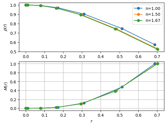
Now let's apply our solver for a range of polytropic indices and see what star radius we obtain.

sols = {}
ns = (1, 3/2., 5/3.)
fig, axs = plt.subplots(2)

for n in ns:
    sols[n] = calculate_star_structure(n)
    axs[0].plot(sols[n].t, sols[n].y[0,:], "-o", label=f"n={n:.2f}")
    axs[1].plot(sols[n].t, sols[n].y[1,:], "-o", label=f"n={n:.2f}")
    
plt.xlabel("$r$")
axs[0].set_ylabel(r"$\rho(r)$")
axs[1].set_ylabel(r"$M(r)$")
axs[0].legend()
axs[1].legend()
plt.grid()

So the radius of the star is for all the considered polytropic models under (the given boundary conditions) roughly equal to 0.7. This doesn't mean that all polytropic stars have the same structure and radius. Depending on the total mass in central density, which may vary depending on what nuclear physics is going on in detail, we would get very different results.

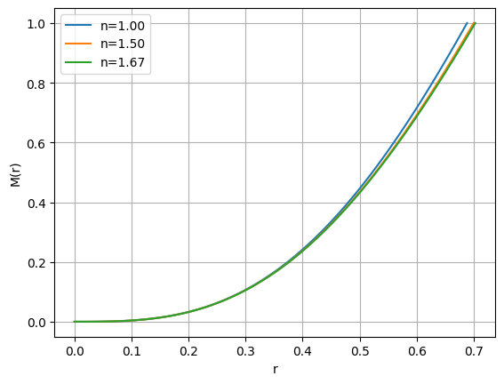
Now that we have an idea of how large the radius is, we can ask the solver for a denser output:

ns = (1, 3/2., 5/3.)
for n in ns:
    R = sols[n].t[-1]
    R0 = sols[n].t[0]
    sols[n] = calculate_star_structure(n, t_eval=np.linspace(R0, R, 100))
    plt.plot(sols[n].t, sols[n].y[1,:], "-", label=f"n={n:.2f}")
    
plt.xlabel("r")
plt.ylabel("M(r)")
plt.legend()
plt.grid()

Conclusion

The exploration of polytropic stars through mathematical modeling and computational techniques gives an intriguing glimpse into understanding stellar structures. By using Python and the SciPy library, we've turned abstract equations into concrete insights into the behavior of stars. Though the polytropic model is a simplification, it provides a solid foundation for further study, both for understanding specific stars and for more advanced astrophysical research.